Every data science project follows the same systematic approach. Today we’ll take a quick tour through all 9 steps using simple examples. This gives you the big picture before we dive deeper in coming days!
flowchart LR
    A["1. Import<br/>📂"] --> B["2. Explore<br/>🔍"] --> C["3. Clean<br/>🧹"]
    C --> D["4. Filter<br/>🎯"] --> E["5. Sort<br/>📊"]
    E --> F["6. Transform<br/>🔄"] --> G["7. Group<br/>👥"]
    G --> H["8. Aggregate<br/>📈"] --> I["9. Visualize<br/>📊"]

    style A fill:#e1f5fe
    style B fill:#e8f5e8
    style C fill:#fff3e0
    style D fill:#f3e5f5
    style E fill:#e0f2f1
    style F fill:#fce4ec
    style G fill:#e8eaf6
    style H fill:#f1f8e9
    style I fill:#fff8e1
Session Goals
Today: Quick overview of all 9 steps with simple examples Days 5-7: Deep dive into specific steps with real data End-of-day: Practice the complete workflow yourself!
Getting Started
Create a new notebook called Session_4C_Workflow_Tour.ipynb and type along as we tour the data science workflow!
Setup
Code
import pandas as pdimport matplotlib.pyplot as plt
Workflow Tour: 9 Simple Steps
Follow along and type each step. We’ll use simple, short commands that are easy to type!
/var/folders/bs/x9tn9jz91cv6hb3q6p4djbmw0000gn/T/ipykernel_230/79280054.py:2: SettingWithCopyWarning:
A value is trying to be set on a copy of a slice from a DataFrame.
Try using .loc[row_indexer,col_indexer] = value instead

See the caveats in the documentation: https://pandas.pydata.org/pandas-docs/stable/user_guide/indexing.html#returning-a-view-versus-a-copy
  df_clean['temp_f'] = df_clean['temperature'] * 9/5 + 32
temperature
temp_f
1
14.800079
58.640143
2
23.752256
74.754061
3
24.702824
76.465082
4
10.244824
50.440683
5
13.489102
56.280384
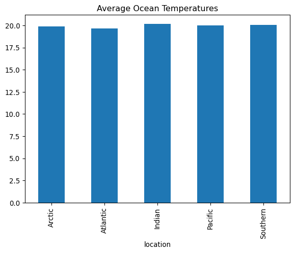
👥 Step 7: Group
Key Function: df.groupby()
Code
# Group databy_ocean = df_clean.groupby('location')by_ocean.size()